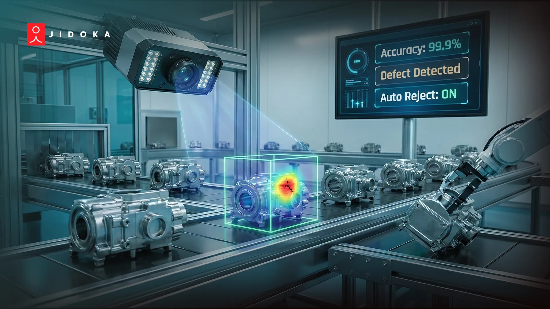
AI defect detection is automated visual inspection where a trained computer vision model decides whether a part passes, instead of a fixed pixel rule. A camera captures each unit, a deep learning model scores the image against thousands of examples of good and bad, and the line acts on that score in milliseconds.
The global AI defect detection market was valued at $3.31 billion in 2024 and is projected to reach $6.63 billion by 2034. The pressure behind that growth is measurable. The American Society for Quality puts the cost of poor quality at 15% to 20% of sales revenue in many plants, and manual inspection is where a large share of it leaks out.
AI quality inspection is now the working baseline for plants competing on both throughput and escape rate. This guide covers the four detection methods, how much labelled data each one needs, what a number like 99.8% accuracy actually measures, why pilots stall before they reach production, and what a live deployment looks like on a real line.
What is AI defect detection?
AI defect detection uses computer vision and deep learning to identify flaws in parts, assemblies, prints, or packaging automatically, without a human inspector and without hand-coded rules. The model learns what acceptable looks like from example images, then scores every unit that passes the camera and sends a pass or reject decision to the PLC in real time.
The difference from traditional machine vision sits in where the decision rule comes from. A rule-based automated optical inspection system is told what to look for as a fixed threshold, and every automated visual inspection recipe has to be written by hand. An AI system is shown examples and learns the boundary itself, which is why it holds up when lighting drifts, surface finish varies, or a new product variant enters the line.
DimensionRule-based machine vision (AOI)AI defect detectionDecision ruleHand-coded thresholds on pixels, edges, blob sizeLearned from labelled or reference imagesNatural product variationTriggers false rejectsTolerated once represented in training dataNew defect typeNeeds manual reprogrammingNeeds new example images and a retrainNew product variantNew recipe built from scratchTransfer from the existing modelReflective, textured, or printed surfacesWeak, high false positive rateHandles once lighting is controlledTypical failure modeRejects good partsMisses defect classes it was never shown
Neither approach replaces the other everywhere. Gauging a hole diameter to a fixed tolerance is still a job for classical metrology. Judging whether a weld bead looks acceptable across six suppliers and three surface finishes is where the learned model earns its place. A fuller side-by-side sits in our breakdown of KOMPASS versus traditional inspection methods.
How does AI actually catch a defect a human inspector misses?
It runs the same five steps on every single unit, at the same standard, for the whole shift. That consistency is the advantage, more than raw resolution, and it is why AI quality inspection catches micro-defects that a tiring eye passes over at line speed.
- Capture. A line-scan or area-scan camera images the part under controlled lighting, timed off an encoder or a proximity trigger.
- Preprocess. The frame is normalised for exposure, aligned to a reference pose, and cropped to the regions that matter.
- Infer. A convolutional or transformer-based model scores the image, returning a class, a bounding box, a pixel mask, or an anomaly score.
- Decide. The score is compared against a calibrated threshold tuned to the plant's tolerance for escapes versus false rejects.
- Act. The verdict goes to the PLC, which fires a reject arm, diverts the unit, or flags the station, and the image is logged for traceability.
A human inspector sees the same part once, for a fraction of a second, on the tail end of a shift, with attention that varies by hour and by operator. The model has no such variance. It also captures every image it judged, which turns inspection into a data stream you can run root cause analysis against instead of a verdict that disappears when the part moves on.
Which defects can AI detect, and which ones still slip through?
Anything that shows a consistent visual signature under the right imaging setup is detectable. The table below maps the families that come up most often on production lines.
Defect familyTypical examplesMethod that usually fitsDifficultySurface flawsScratches, dents, pits, burrs, corrosion, coating runsSegmentation or anomaly detectionModerate, lighting-sensitivePrint and labelMissing text, smudged code, wrong orientation, OCR mismatchObject detection plus OCRLow once fonts are coveredPresence and assemblyMissing fastener, wrong connector, out-of-sequence stepObject detectionLow to moderateDimensional and geometricGap and flush, warp, flatness, misalignment3D imaging plus measurementModerate, needs calibrated opticsFill and sealUnder-fill, cap tilt, seal leak, crimp failureClassification or 3D profilingLow to moderateContaminationForeign object, debris, hair, particulateAnomaly detectionHigh, defects are rare and variedSubsurfaceInternal voids, porosity, micro-cracks under coatingX-ray, thermal, or ultrasonic imagingHigh, optical cameras cannot see it
Three limits are worth stating plainly, because they are what separate a pilot that works from one that quietly fails.
- Nothing beneath the surface, without the right sensor. A visible-light camera cannot find a void inside a casting. That needs X-ray or thermography feeding the same model pipeline.
- Nothing the model has never seen, unless it is running anomaly detection. A supervised classifier trained on scratches and dents will happily pass a defect type nobody labelled.
- Nothing that is invisible at the chosen resolution and lighting. Micro-defect detection at 50 microns is an optics and lighting problem first, and a model problem second.
Deeper walkthroughs by family sit in our guides to presence inspection, web inspection defects, and flatness measurement using 3D vision.
Classification, detection, segmentation, or anomaly detection: which one does my line need?
Pick the method by the answer the line needs, not by which architecture sounds strongest. A reject arm only needs pass or fail. A process engineer chasing a die wear trend needs the defect outlined and measured.
MethodWhat it returnsTraining data it needsUse it whenImage classificationOne label for the whole image, such as pass or crackLabelled examples of every classThe decision is binary and the defect is always in frameObject detectionBoxes around each defect, with a class and countBox annotations per defect instanceYou need to know how many and roughly whereSemantic segmentationA pixel mask outlining the defectPixel-level masks, the most costly to labelArea, length, or shape drives the accept or reject callAnomaly detectionA deviation score against a learned normalMostly good parts, few or no defect imagesDefects are rare, varied, or not yet catalogued
Real deployments usually combine them. A fast classifier gates the line, segmentation runs on flagged units to size the defect, and an anomaly detection layer stays on top to catch the class nobody has seen yet. That third layer is what stops a supervised model from confidently passing a brand new failure mode.
How many defect images do I actually need to train it?
It depends entirely on the method, and the honest range runs from almost none to several thousand per class. Anomaly detection needs mainly good parts, which most plants already have thousands of. Conventional supervised training needs hundreds to low thousands of labelled images per defect class. Transfer learning and few-shot pipelines bring that down sharply, into the tens per class, because the model starts from features learned elsewhere and only adapts the final layers.
The real constraint is rarely total volume. It is class imbalance. On a well-controlled line, the defect you most want to catch may occur at a few dozen parts per million, so waiting for enough natural examples would take months of production. Working teams get around this by seeding the training set with deliberately produced defective samples, by augmenting the images they do have, or by inverting the problem and modelling normal instead.
On Jidoka deployments, new product variants typically come online with 60% to 70% fewer training samples than a fresh model would need, because the variant inherits from the existing model rather than starting over. That number matters more than a headline accuracy figure when a plant runs a high-mix schedule and adds variants every quarter.
What does 99.8% accuracy actually mean?
On its own, an accuracy percentage tells you very little, and vendors quote it because it sounds decisive. If 99.5% of the parts coming down the line are good, a model that passes everything scores 99.5% accuracy and catches nothing. The metrics that decide whether a system is worth installing are these four.
MetricThe question it answersWhy it matters on the lineRecall (detection rate)Of all real defects, how many did we catch?Low recall means escapes reach the customerPrecisionOf everything we rejected, how many were truly defective?Low precision means good parts scrapped and operators overriding the systemEscape rate in PPMHow many defective parts per million shipped?The number your customer's quality agreement is actually written againstGauge R&RDoes the system give the same verdict on the same part, every time?Required evidence under IATF 16949 and similar standards
Recall and precision trade against each other, and the threshold that balances them is a business decision rather than a technical one. A pharmaceutical line will accept extra false rejects to drive escapes toward zero. A high-volume consumer goods line cannot afford to scrap 3% of good output and will tune the other way.
When Jidoka reports 99.8% or better, it refers to sustained performance on live production lines under normal shift conditions, measured against operator-verified ground truth, not a benchmark run on a curated image set. That distinction is the one to press every vendor on, including us. Ask what the number measures, on which line, over how many parts, and against whose ground truth. The accuracy benchmark methodology is worth reading before any pilot is signed off.
Why do AI inspection projects stall after the pilot?
From what we see across plants, the model is almost never the reason. Pilots run on clean images, in a quiet corner, with an engineer watching. Production is a different environment, and the failures cluster into five patterns.
- Lighting and fixturing drift. A lamp ages, a fixture shifts by two millimetres, or sunlight reaches the station in July. Accuracy falls and nobody connects it to the cause.
- No retraining loop. The model was trained once against a golden sample set and never updated as suppliers, tooling, and finishes changed underneath it.
- False rejects destroying trust. Once operators start overriding the system because it scraps good parts, the installation is finished, whatever the dashboard says.
- Results with nowhere to go. Verdicts land in a web dashboard instead of the PLC and the MES, so nothing on the floor actually changes.
- Rare classes with too few examples. The defect that triggered the project happens 40 times a million and never accumulated enough images to train against.
Every one of these is an integration and process problem rather than an algorithm problem. Budgeting for camera and lighting engineering, a retraining cadence, and PLC integration is what carries a pilot into production.
Where AI defect detection is already running
Automated visual inspection requirements differ sharply by industry, though the underlying goal stays the same across all of them: zero escapes at full line speed.
Semiconductor and electronics
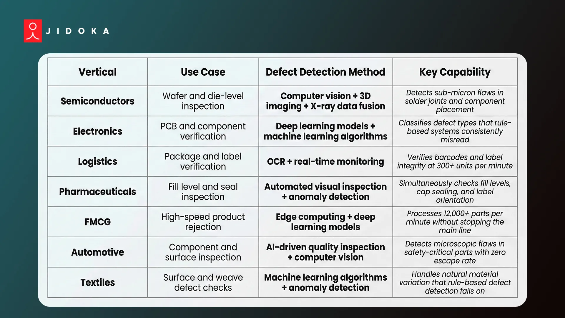
Defects here can be smaller than a human hair. Automated inspection systems combine 3D imaging with X-ray data to verify solder joints and component placement in milliseconds. Models trained on wafer map data classify failure signatures that older CNN architectures consistently confuse, and NVIDIA has published work on vision foundation models for exactly this classification problem. A single escape in mission-critical hardware costs more downstream than the entire inspection system. Solder paste inspection is usually the first station to automate.
Automotive and metal parts
Automotive lines carry the heaviest documentation burden of any vertical. Detection has to hold across supplier variation in castings, stampings, and welds, and the system itself has to pass gauge studies before it can be trusted as a control. Our guide to automotive quality control under IATF 16949 covers what auditors expect from an AI inspection station, and automotive deployments typically start at weld, paint, or final assembly verification.
High-speed logistics and sorting
In warehousing and logistics, inspection extends past broken packaging into identity. OCR verification runs at over 300 units per minute, reading through print variation, contamination, and surface noise. Misread frames feed back into the training set automatically, so recognition improves with every cycle instead of degrading.
FMCG, food, and pharmaceutical packaging
Pharmaceutical lines carry a near-zero tolerance for error, and a single inspection station checks fill level, cap seal, and label orientation at the same time. In FMCG production, models on edge hardware clear thousands of units per minute and reject defective items without stopping the main line, while anomaly detection catches the deviations fixed-threshold systems were never configured to see.
Should inference run at the edge or in the cloud?
At the edge, for anything that has to trigger a physical reject. A line moving at several metres per second gives the system a decision budget in the low tens of milliseconds, and a cloud round trip cannot meet it. Edge inference on a local GPU or accelerator keeps the loop closed between camera, model, and PLC.
Two further reasons push the same way. Production imagery often carries competitive or regulated information, and keeping it on-premises removes an entire data governance conversation. Edge deployment also keeps the line inspecting during a network outage, which is not a rare event in a plant.
Cloud still has a role, on the training side. Retraining a model on months of accumulated images is a batch job with no latency requirement, and it belongs where the compute is cheap. The pattern that works is train centrally, infer locally.
The next step beyond that is agentic behaviour. Instead of raising a dashboard alert when a scratch pattern repeats, the system signals the upstream machine to recalibrate or holds the line before defective parts multiply. Siemens runs this on Armv9-based edge platforms, correcting component defects ahead of final inspection. That closes the loop from detection into prevention.
What does it take to get one line live?
A single-line deployment commonly runs six to ten weeks from site survey to production sign-off, with variant count and defect rarity driving most of the variance. The sequence looks like this.
- Site survey and imaging design. Defect list, resolution target, camera and lens selection, lighting geometry, trigger source, and cycle time budget.
- Hardware install and image collection. Cameras and lighting mounted and locked down, then production images captured across shifts, suppliers, and variants.
- Labelling and model training. Ground truth agreed with the quality team, defect classes defined, model trained, and the accept threshold calibrated against the plant's escape and false-reject tolerance.
- Integration. Verdicts wired into the PLC for physical rejection and into the MES or quality system for traceability, with images retained against each serial.
- Run-in and handover. Shadow operation alongside human inspection, gauge study, threshold tuning, and a documented retraining cadence handed to the plant team.
Plants that already have camera infrastructure in place can compress the first two phases considerably.
How Jidoka runs defect detection at 12,000 parts a minute
Detection under real production pressure needs cameras, lighting, PLC timing, and edge compute working together across every shift. Jidoka Technologies builds that full stack, and plants running it sustain automated inspection at 12,000+ parts per minute and up to 300 million inspections per day.
Two systems carry the load.
1. KOMPASS, the high-accuracy inspector
- Sustains 99.8%+ accuracy on live production lines, measured against operator-verified ground truth
- Scores each frame in under 10ms, inside the reject-arm timing budget
- Brings new variants online with 60% to 70% fewer training samples
- Handles reflective metal, printed surfaces, and textured parts that defeat threshold-based systems
2. NAGARE, the process and assembly analyst
- Tracks 100% of assembly steps through cameras the plant already has
- Flags missing parts and out-of-sequence operations as they happen, rather than at final inspection
- Cuts rework by 20% to 35% across industrial deployments
Both run entirely on local edge units, which keeps the decision, the latency, and the image data on the floor where they belong. Together they move a plant toward right first time rather than catch-and-rework, which is where the cost of poor quality actually comes down.
Want to see how this performs on your line? Book an assessment with Jidoka and we will map where your current inspection process is losing yield.
Frequently asked questions
How accurate is AI defect detection compared with manual inspection?
AI inspection holds a constant standard across the whole shift, which is where manual inspection loses ground. Human accuracy varies by hour, operator, and line speed, while a trained model applies the identical threshold to every unit and logs the image behind each verdict. Jidoka's KOMPASS sustains 99.8% or better on live lines. The figure to compare across vendors is recall and escape rate in PPM, not a headline accuracy percentage.
Can AI defect detection work with the cameras and PLCs I already have?
Usually yes. Modern systems are hardware-agnostic and connect to existing industrial cameras, PLCs, and conveyors through an edge gateway, so the plant is not replacing its automation layer. The component most often needing an upgrade is lighting rather than compute, because consistent illumination determines whether the defect is visible to the model at all. Our guide to industrial cameras for defect detection covers when existing optics are good enough.
How many images do I need before the system is production ready?
Anomaly detection needs mainly good parts, which most plants already hold in volume. Supervised classification needs hundreds to low thousands of labelled images per defect class, and transfer learning brings that into the tens. Class imbalance is the harder constraint, so teams working with rare defects seed the set with deliberately produced samples instead of waiting for natural occurrence.
What is the difference between AI defect detection and traditional machine vision?
Traditional automated optical inspection applies hand-coded thresholds and rejects anything outside them, so natural product variation reads as a defect. AI defect detection learns the boundary between good and bad from example images, which lets it hold accuracy across lighting changes, surface finishes, and new product variants without a fresh recipe being written each time.
Which defects can AI not detect?
Three categories stay out of reach. Subsurface flaws such as internal voids and porosity need X-ray, thermal, or ultrasonic imaging rather than a visible-light camera. Defect types the model was never shown will pass unless an anomaly detection layer is running alongside the classifier. Anything below the resolution or contrast the optics can resolve is an imaging problem before it is a model problem.
What is agentic AI in defect detection?
Agentic AI acts on the detection rather than reporting it. When a defect pattern repeats, the system recalibrates the upstream machine or holds the line on its own instead of waiting for a human to read a dashboard alert. This turns inspection from a record of what went wrong into a control that stops the next unit from going wrong.
Does AI defect detection run on the edge or in the cloud?
Inference runs at the edge, because triggering a physical reject leaves a decision budget in the low tens of milliseconds and a cloud round trip cannot meet it. Training and retraining run centrally, where batch compute is cheap and latency is irrelevant. Edge inference also keeps production imagery on-premises and keeps the line inspecting through a network outage.
How long does it take to deploy AI defect detection on one line?
A single line commonly takes six to ten weeks, covering site survey and imaging design, hardware installation and image collection, labelling and model training, PLC and MES integration, then a shadow run alongside human inspection before sign-off. Plants with usable camera infrastructure already installed compress the early phases considerably.